
Morphological Transformations in Python using OpenCV
in Image Processing, Python on November 22, 2020by coseriesMorphological transformations are those non-linear operations that are based on image shape. They require an input image and a structuring element. Moreover, they return an output image after applying the structuring element on the input image. Morphological operations are often applied to binary images, but we can perform them on grayscale images as well. In this article, we will go through different morphological operations such as erosion, dilation, opening, and closing, etc. The last article of this series was on Image Thresholding. If you are new here, you can visit our previous articles.
Structuring Element
So, what is a structuring element? A structuring element or a kernel is a small shape or a matrix that determines the value of the image pixel being processed and the neighborhood that is taken into consideration, just like kernels (filters) do in the image smoothening. It is usually an odd-sized kernel and contains binary values, i.e., 0 and 1. The pattern of 0 (black) and 1 (white) determines its shape. For example, a structuring element with all the values equal to 1 has the shape of a rectangle.
Erosion
Erosion is an operation in morphological transformation that shrinks or thins objects in a binary image. It increases the gap between different regions and removes details that are smaller than the structuring element.
How does it work?
Let our input image be I and the structuring element be B. B slides over every possible pixel of image I. A pixel at the position (x, y) will retain its value, if for each of the pixels in the B equal to 1, the corresponding pixel in the image I is also 1. Otherwise, the pixel at the position (x, y) will get eroded, i.e., will be assigned a zero value.
It erases the boundaries of a foreground object. Note that here, the foreground is considered to be white. So, let’s say when a rectangular structuring element is positioned at a boundary pixel of an object, some of the pixel values under the kernel will be black (background). Therefore, that boundary pixel will become zero.
cv2.getStructuringElement()
OpenCV provides the cv2.getStructuringElement() function to obtain the kernel. It takes the desired shape and the size of the kernel. OpenCV provides the following shapes:
- cv2.MORPH_RECT
- cv2. MORPH_CROSS
- cv2.MORPH_ELLIPSE
cv2.erode()
To apply the erosion, OpenCV provides the cv2.erode() function. It takes two required arguments: an image and a structuring element. The default anchor position is at the center of the kernel, i.e., (-1, -1). If you want to change it, you can provide the anchor argument. You can also apply the same structuring element multiple times by providing the iterations (default value is 1) argument. Moreover, it takes borderType and borderValue to specify the type of the border and the value if the border is constant. The default border type is cv2.BORDER_CONSTANT.
Consider the following example.
import cv2

img = cv2.imread("morph.png", 0)
kernel = cv2.getStructuringElement(cv2.MORPH_RECT, (9,9))
print(kernel)
eroded_img = cv2.erode(img, kernel)
cv2.imshow("Original image", img)
cv2.imshow("Eroded image", eroded_img)
cv2.waitKey(0)
cv2.destroyAllWindows()
Output
[[1 1 1 1 1 1 1 1 1]
 [1 1 1 1 1 1 1 1 1]
 [1 1 1 1 1 1 1 1 1]
 [1 1 1 1 1 1 1 1 1]
 [1 1 1 1 1 1 1 1 1]
 [1 1 1 1 1 1 1 1 1]
 [1 1 1 1 1 1 1 1 1]
 [1 1 1 1 1 1 1 1 1]
 [1 1 1 1 1 1 1 1 1]]
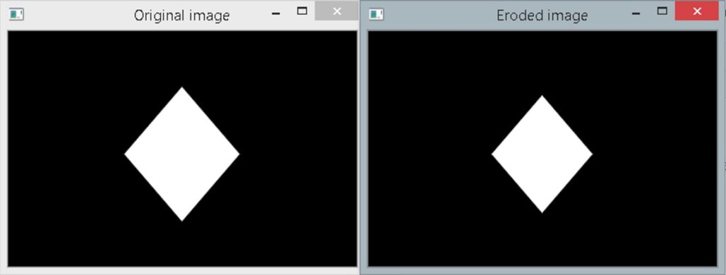
In the above example, we apply a rectangular structuring element of size 9 by 9 on the image. As you can see in the output above, the object is shrunk (boundary pixels get eroded) after performing the erosion operation.
Let’s look at another example.
import cv2

img = cv2.imread("morph1.png", 0)
kernel = cv2.getStructuringElement(cv2.MORPH_RECT, (9,9))
print(kernel)
eroded_img = cv2.erode(img, kernel)
cv2.imshow("Original image", img)
cv2.imshow("Eroded image", eroded_img)
cv2.waitKey(0)
cv2.destroyAllWindows()
Output
[1 1 1 1 1 1 1 1 1]
 [1 1 1 1 1 1 1 1 1]
 [1 1 1 1 1 1 1 1 1]
 [1 1 1 1 1 1 1 1 1]
 [1 1 1 1 1 1 1 1 1]
 [1 1 1 1 1 1 1 1 1]
 [1 1 1 1 1 1 1 1 1]
 [1 1 1 1 1 1 1 1 1]]
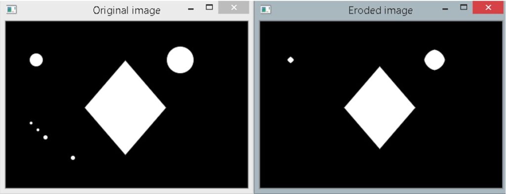
As you can observe in the above example, objects having sizes smaller than the structuring element get completely erased, while others get shrunk.
Dilation
It is the opposite of erosion. It expands or thickens objects in images. With dilation, you can fill up or reduce small holes in an object.
How does it work?
Let our input image be I and the structuring element be B. B slides over every possible pixel of image I. A pixel at the position (x, y) will take the value 1, if for any of the pixel in the B equal to 1, the corresponding pixel in the image I is also 1. Otherwise, the pixel at the position (x, y) will get a zero value.
Opposite to erosion, dilation thickens the boundary of a foreground (white) object. Consider a rectangular structuring element positioned at an object’s boundary pixel, which has the value 1. So, after applying dilation, it will retain that value. Moreover, if we have a pixel just outside the boundary pixel, it will become 1 because the boundary pixels will come under the kernel, and they have the value 1. In this way, the size of an object gets increased. Moreover, the amount of thickening depends upon the kernel size.
cv2.dilate()
The cv2.dilate() function is used to perform the dilation operation. The two required arguments are an image and a structuring element. Just like cv2.erode(), it also takes an anchor position, iterations, borderType, and borderValue.
Consider the following example.
import cv2

img = cv2.imread("morph.png", 0)
kernel = cv2.getStructuringElement(cv2.MORPH_CROSS, (9,9))
print(kernel)
dilated_img = cv2.dilate(img, kernel)
cv2.imshow("Original image", img)
cv2.imshow("Dilated image", dilated_img)
cv2.waitKey(0)
cv2.destroyAllWindows()
Output
[[0 0 0 0 1 0 0 0 0]
 [0 0 0 0 1 0 0 0 0]
 [0 0 0 0 1 0 0 0 0]
 [0 0 0 0 1 0 0 0 0]
 [1 1 1 1 1 1 1 1 1]
 [0 0 0 0 1 0 0 0 0]
 [0 0 0 0 1 0 0 0 0]
 [0 0 0 0 1 0 0 0 0]
 [0 0 0 0 1 0 0 0 0]]
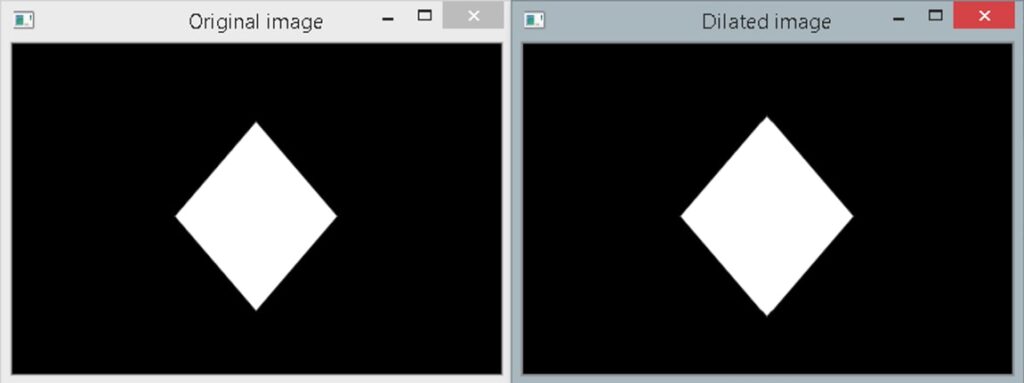
In the above example, we apply a 9 by 9 cross-shaped structuring element. Since our object is of the diamond-shaped, a better approach would be to apply the kernel of the same shape as well. However, OpenCV does not provide that shape, so we can create our structuring element using the NumPy array or some external library. Consider the following example in which we use the scikit-image library to get the diamond-shaped structuring element.
import cv2
from skimage import morphology
img = cv2.imread("morph.png", 0)
kernel = morphology.diamond(4)
print(kernel)
dilated_img = cv2.dilate(img, kernel)
cv2.imshow("Original image", img)
cv2.imshow("Dilated image", dilated_img)
cv2.waitKey(0)
cv2.destroyAllWindows()
Output
[[0 0 0 0 1 0 0 0 0]
 [0 0 0 1 1 1 0 0 0]
 [0 0 1 1 1 1 1 0 0]
 [0 1 1 1 1 1 1 1 0]
 [1 1 1 1 1 1 1 1 1]
 [0 1 1 1 1 1 1 1 0]
 [0 0 1 1 1 1 1 0 0]
 [0 0 0 1 1 1 0 0 0]
 [0 0 0 0 1 0 0 0 0]]

Here, we use morphology.diamond() function to get the desired kernel. It takes a radius and dtype (default value is np.uint8). To learn more, visit here. Consider the following example in which we fill up the holes in an object by performing dilation.
import cv2
img = cv2.imread("morph3.png", 0)
kernel = cv2.getStructuringElement(cv2.MORPH_CROSS, (11,11))
dilated_img = cv2.dilate(img, kernel)
cv2.imshow("Original image", img)
cv2.imshow("Dilated image", dilated_img)
cv2.waitKey(0)
cv2.destroyAllWindows()
Output
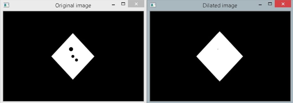
As you can see in the output above, the gaps got almost filled. Moreover, the size of the object gets increased as well.
Opening
Erosion and dilation are two basic operations in morphological transformation. Other operations are obtained from their combination, such as opening, closing, and gradient, etc.
Opening is a compound morphological operation. It is achieved by first eroding the image and then dilating it. When we first erode an image, it removes small white noises but decreases the size of larger objects as well. So, by applying dilation, the larger objects get back to its original size.
cv2.morphologyEx()
The cv2.morphologyEx() is used to perform compound morphological operations. It takes an image, type of the operation, kernel, anchor position, iterations, borderType, and borderValue. To perform opening, pass cv2.MORPH_OPEN as the operation type.
Consider the following example.
import cv2
img = cv2.imread("morph2.png", 0)
kernel = cv2.getStructuringElement(cv2.MORPH_RECT, (9,9))
opening = cv2.morphologyEx(img, cv2.MORPH_OPEN, kernel)
cv2.imshow("Original image", img)
cv2.imshow("Opening", opening)
cv2.waitKey(0)
cv2.destroyAllWindows()
Output

As you can see in the output above, the small details get removed, but the size of the rectangle remains the same.
Closing
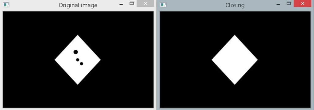
It is the opposite of the opening. In closing, erosion follows dilation. It fills up gaps in an object while keeping its size the same.
To perform the closing operation, pass cv2.MORPH_CLOSE as the operation type in the cv2.morphologyEx() function. Let’s see.
import cv2
img = cv2.imread("morph3.png", 0)
kernel = cv2.getStructuringElement(cv2.MORPH_RECT, (11, 11))
closing = cv2.morphologyEx(img, cv2.MORPH_CLOSE, kernel)
cv2.imshow("Original image", img)
cv2.imshow("Closing", closing)
cv2.waitKey(0)
cv2.destroyAllWindows()
Output
Morphological Gradient
The gradient is the difference between the dilation and the erosion of an image. When we dilate an image, the boundary of an object increases, and eroding an image decreases it. So, when we take the difference, we are left with the outline of an object only. Pass cv2.MORPH_GRADIENT in the cv2.morphologyEx() function to perform the gradient operation. Let’s see.
import cv2
img = cv2.imread("morph4.png", 0)
kernel = cv2.getStructuringElement(cv2.MORPH_RECT, (3,3))
gradient = cv2.morphologyEx(img, cv2.MORPH_GRADIENT, kernel)
cv2.imshow("Original image", img)
cv2.imshow("Gradient", gradient)
cv2.waitKey(0)
cv2.destroyAllWindows()
Output

As you can see, we get the boundary or an outline of the object when we perform the gradient operation.
Black Hat or Bottom Hat
It is the difference between the input image and its closing. For the bottom hat operation, use cv2.MORPH_BLACKHAT. Let’s see.
import cv2
img = cv2.imread("morph3.png", 0)
kernel = cv2.getStructuringElement(cv2.MORPH_RECT, (11,11))
black_hat = cv2.morphologyEx(img, cv2.MORPH_BLACKHAT, kernel)
cv2.imshow("Original image", img)
cv2.imshow("Black Hat", black_hat)
cv2.waitKey(0)
cv2.destroyAllWindows()
Output
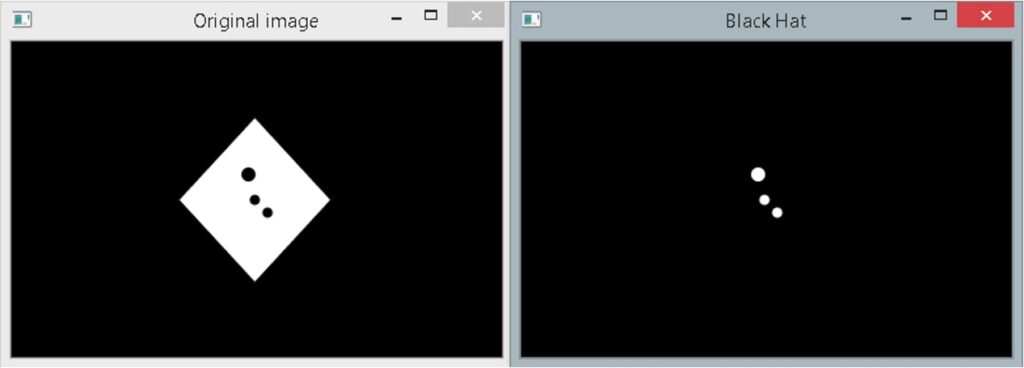
When we performed the closing operation on the same image, i.e., morph3.png in the above section, the holes inside the diamond-shaped object got filled. If we subtract that closed image from the input image, we will get the holes only, which are shown in the output above.
Top Hat
It is the difference between the input image and its opening. For the top hat operation, use cv2.MORPH_TOPHAT. Consider the example below.
import cv2
img = cv2.imread("morph2.png", 0)
kernel = cv2.getStructuringElement(cv2.MORPH_RECT, (9,9))
top_hat = cv2.morphologyEx(img, cv2.MORPH_TOPHAT, kernel)
cv2.imshow("Original image", img)
cv2.imshow("Top Hat", top_hat)
cv2.waitKey(0)
cv2.destroyAllWindows()
Output


