Image Smoothing (Blurring) in Python Using OpenCV
in Python, Image Processing on November 17, 2020by coseriesImage blurring or smoothing is quite an important topic in image processing. When we blur an image, the details in it get reduced. Image blurring has many applications. For example, you must have observed some people or things blurred in a video or an image to hide information. The blur feature that you use to blur your photos is another application. It is also used in removing noise. When you have a noisy pixel in an image, it represents an outlier, i.e., its intensity is distinct from its neighborhood. So, whenever we have noise, it shows a sharp intensity transition. When we smoothen an image, these transitions are scaled-down. In this article, we will learn how to perform image smoothing using various low-pass (smoothing) filters.
What is a Filter?
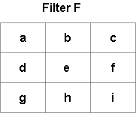
As mentioned above, we need to apply specific filters to images to perform blurring. A filter or a kernel is an array of size m by n, where m and n are both odd numbers. Consider the figure below.
Convolution
This is a filter (kernel) F of size 3 by 3. Now, to apply the filter F to image I, do the following for each image pixel (x, y):
- Flip the kernel by 180o. If it is symmetrical, there is no need to do that.

- Align the center of the filter F with the position (x, y).
- Take the sum of products of the filter F and the image I at (x, y). Consider the figure below to understand the concept.
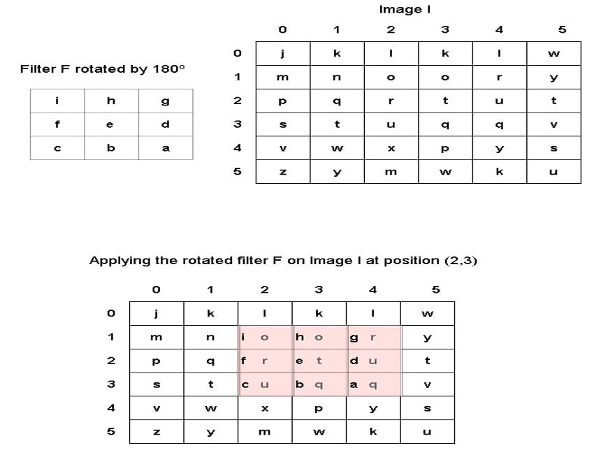
In the figure above, we apply the filter at the position (2, 3) of the image I. As you can observe, the center of the kernel is aligned with (2, 3). We multiply corresponding numbers, i.e., e × t, and then sum them up. The new value at the position (2, 3) will be:
I’ (2, 3) = i × o + h × o + g × r + f × r + e × t + d × u + c × u + b × q + a × q
Moreover, a – i letters are the coefficients of the filter and are real numbers. The letters j-z, on the other hand, represent intensity values.
The above operation is known as the convolution.
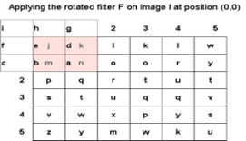
What happens if we apply the filter on the boundaries, for example, at the position (0, 0). As you can see in the figure below, some part of the filter is outside the image, and hence, we cannot perform convolution. To solve that problem, we can add padding (borders) around the edges.
The cv2.filter2D() function
OpenCV provides us the cv2.filter2D() function to convolve a filter with an image. It takes an image, depth of the output image (You can pass -1 to use the depth of the source image.), and the filter. It also takes other optional arguments such as the anchor position and the borderType. By default, anchor = (-1, -1), you can change it as well. Consider the figure below for the anchor positions of a 3 by 3 kernel.
| 0 | -1 | 1 | |
| 0 | a | b | c |
| -1 | d | e | f |
| 1 | g | h | I |
By default, the borderType is cv2.BORDER_DEFAULT or cv2.BORDER_REFLECT_101. To learn about various border flags and what they do, visit this.
Consider the following example.
import cv2
import numpy as np
img = cv2.imread("car_img.jpg", 1)

kernel = np.ones((3,3),np.float32)/9
dst = cv2.filter2D(img,-1,kernel, borderType=cv2.BORDER_DEFAULT)
cv2.imshow("Original image", img)
cv2.imshow("Blurred Image", dst)
cv2.waitKey(0)
cv2.destroyAllWindows()
Output
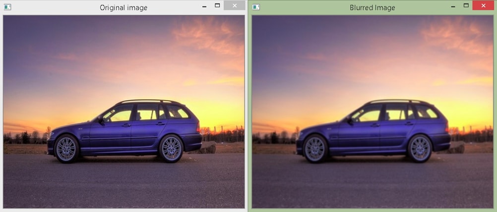
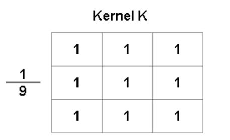
In the above example, we create a 3 by 3 kernel using the np.ones() method, which means every element has the value 1. Then, we divide it by 9. Now, each element has the value 1/9. The kernel is given below.
Averaging
The above type of filter is known as the box filter or the mean filter. It has all the weights or coefficients equal to 1. Moreover, we divide the kernel by the sum of its weights to normalize it, i.e., the sum of all the elements is equal to 1. We are doing averaging here. When we convolve the image with this kernel, it sums the pixel values in the 3 by 3 neighborhood and then divides it by the total number of pixels, i.e., 3×3 = 9. As you can see in the output above, the car image after applying the filter gets blurred.
Let’s now apply a filter of size 7 by 7.
import cv2
import numpy as np
img = cv2.imread("car_img.jpg", 1)

kernel = np.ones((7,7),np.float32)/49
dst = cv2.filter2D(img,-1,kernel)
cv2.imshow("Original image", img)
cv2.imshow("Blurred Image", dst)
cv2.waitKey(0)
cv2.destroyAllWindows()
Output

As we increase the size of the filter, the neighborhood also increases, and thus, more number of pixels start affecting the value at the anchor point. Therefore, the smoothing effect increases.
The cv2.blur() function
For the averaging filter, OpenCV provides a separate function known as cv2.blur(). It takes an image and a tuple containing the filter size. It contains other optional arguments like anchor and borderType as well. Let’s do the same example using cv2.blur().
import cv2
import numpy as np
img = cv2.imread("car_img.jpg", 1)

dst = cv2.blur(img,(7,7))
cv2.imshow("Original image", img)
cv2.imshow("Blurred Image", dst)
cv2.waitKey(0)
cv2.destroyAllWindows()
Output
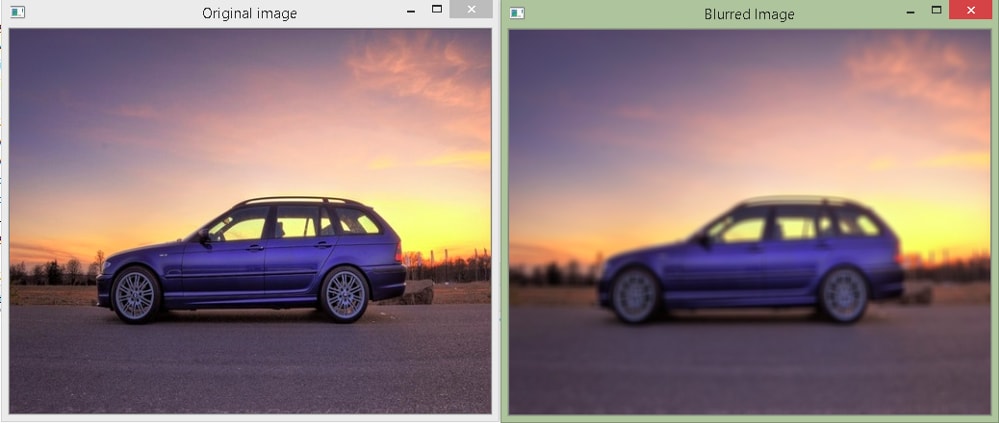
As you can see, we get the same output. However, we do not need to create the filter separately here as we had to when using the cv2.filter2D() function in the example above.
The cv2.boxFilter() function
The cv2.boxFilter() function is almost the same as the cv2.blur() function. However, it allows us to use the unnormalized box filter by passing a keyword argument normalize=False. It also takes an argument for the depth of the output image. Let’s see.
import cv2
import numpy as np
img = cv2.imread("car_img.jpg", 1)

dst = cv2.boxFilter(img,-1,(3,3), normalize=False)
cv2.imshow("Original image", img)
cv2.imshow("Blurred Image", dst)
cv2.waitKey(0)
cv2.destroyAllWindows()
Output
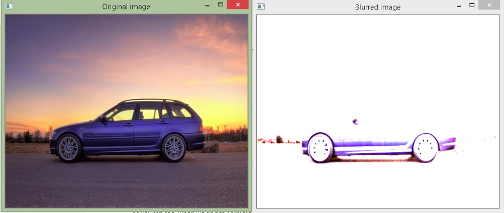
As you can see, when we do not normalize the filter, all the pixel values are just added, which increases the brightness.
Gaussian Filtering
The box filter assigns the same weights to all pixels that comes in its range. So, pixels that are farther from the central pixel have the same effect as the pixels near it. Hence, providing more blurring. Gaussian filter, on the other hand, uses a Gaussian function, and therefore, the weight assigned to the pixel near the anchor point is more than the weight assigned to the distant one. Hence, the effect of pixels decreases as the distance from the center increases. It smoothens sharp edges in the image while reducing extra blurring.
The cv2.GaussianBlur() function
OpenCV provides the cv2.GaussianBlur() function. It takes an image, a tuple containing the kernel size, standard deviation along the x-axis (sigma_x) and the y-axis (sigma_y), and the borderType. If you do not provide sigma_y, then the default value is taken, i.e., 0, which means that it will take the value of sigma_x. If you set sigma_x and sigma_y to 0, then both are calculated automatically from the kernel size.
Consider the following example.
import cv2
import numpy as np
img = cv2.imread("car_img.jpg", 1)

dst = cv2.GaussianBlur(img,(7,7), 0)
cv2.imshow("Original image", img)
cv2.imshow("Gaussian Blur Image", dst)
cv2.waitKey(0)
cv2.destroyAllWindows()
Output
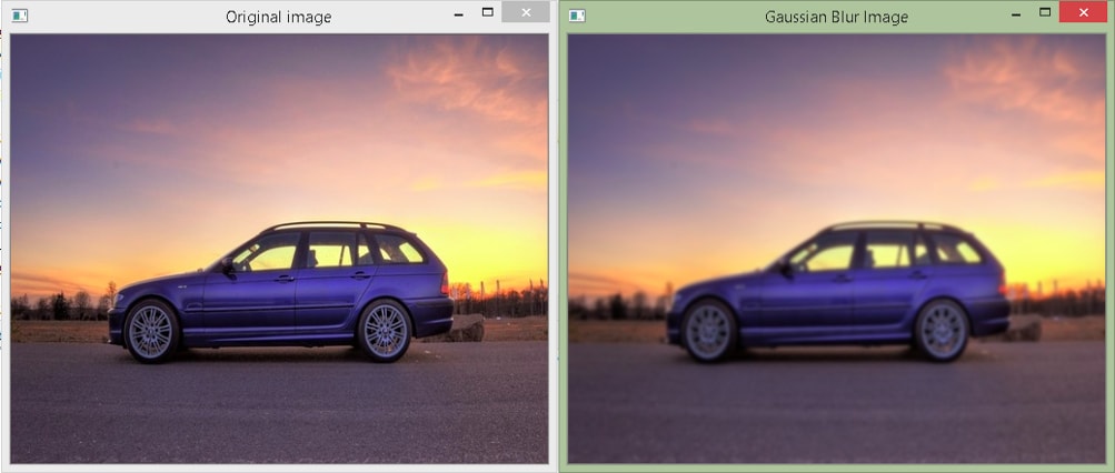
Here, we have taken a kernel of size 7 by 7. Compare its output with the results of the 7 by 7 box filter and observe it is less blurry.
Median Filtering
The median filter computes the median value of the pixels that come under the kernel and replaces the central pixel with that value. It is quite effective in removing salt and pepper noise from images. The salt and pepper noise (or the impulse noise) degrades an image by varying few pixel values with two extremes, 0 and 255. Therefore, when we take the median, these noisy pixels are ordered at ends, and thus, they get removed.
Unlike the mean filter and the Gaussian filter, the new central value taken is always from the existing image pixel. That is why the noise gets removed effectively.
The cv2.medianBlur() function
The cv2.medianBlur() function is used to apply the median filter. It takes an image and the kernel size. Note that the number of rows needs to be equal to the number of columns for the median filter, so we have to pass an odd integer for the size.
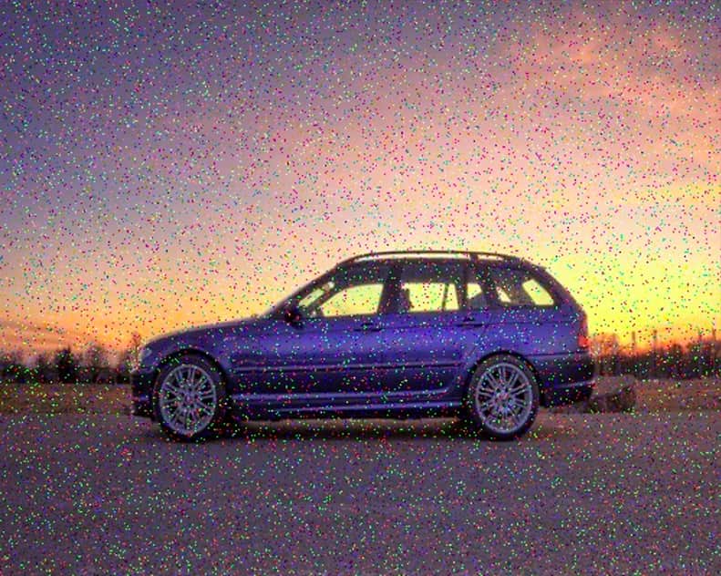
Let’s apply the median filter on the same car image. However, it is corrupted with salt and pepper noise.
import cv2
import numpy as np
img = cv2.imread("car_noise.jpg", 1)

dst = cv2.medianBlur(img,3)
cv2.imshow("Original image", img)
cv2.imshow("Median Blur Image", dst)
cv2.waitKey(0)
cv2.destroyAllWindows()
Output
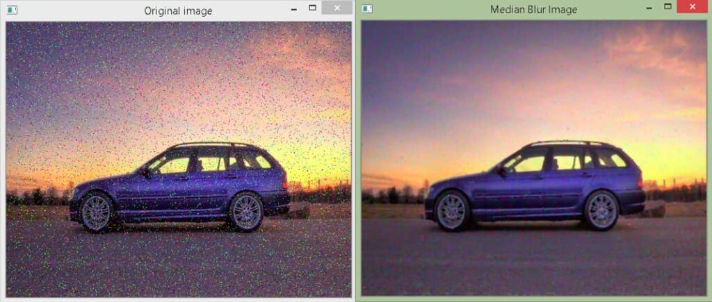
As you can see, most of the noise gets removed by using the median filter of size 3 by 3.

