
In image processing, a histogram is quite an important tool. It provides us a graphical representation of the intensity distribution of an image. On the x-axis, it contains the pixel values that range from 0-255, and on the y-axis, it has the frequency of these pixels, i.e., the number of times each intensity value has occurred.
A histogram can be calculated for both grayscale and color images. However, one histogram can only contain a single channel. Therefore, since grayscale images have only one channel, so they will have one histogram. But color images will require three histograms, one for each channel. For example, for the RGB image, one histogram for the red channel, one for the blue, and one for the green channel.
So why do we need histograms? As already mentioned, a histogram provides us information about the intensity distribution of an image. Moreover, it gives us an idea about the contrast and brightness of the image as well. Histograms also help in finding the threshold value that is used in image segmentation, and edge detection, etc. In this article, we are going to learn about Image Histograms in OpenCV Python.
Histogram Calculation and Visualization
OpenCV provides a function cv2.calcHist() for histograms. It takes the following arguments.
- images: It represents our input image. It should be wrapped up as a list, i.e., [img].
- channels: It represents the index of the channel wrapped up as a list. For grayscale images, pass [0] here. For BGR images, pass [0], [1], or [2] for blue, green, or red channel, respectively.
- mask: It is optional. It is used to plot a specific region of an image.
- histSize: Just like in any other histogram, we can display frequency for a group of pixel values as well, i.e., dividing the pixel values into bins (a series of an interval of values). For example, if the histSize or bin count is eight, then the frequency will be displayed for these eight intervals, and each interval will contain 32 intensity values, i.e., 0-31, 32-63, …,223-255. If you want to find the frequency for each pixel separately, then pass 256 in square brackets, i.e., [256].
- ranges: it shows the range of possible intensity values. It is [0, 256], normally. Here, 256 is not included.
The cv2.calcHist() returns a NumPy array with a shape (histSize, 1). For example, histogram[2][0] returns the frequency of the 2nd bin.
The above method only calculates the histogram, but how do we plot it? For that, we will use the plot() function in the pyplot module of the matplotlib library.
Let’s plot the histogram of the following image and analyze it.

import cv2
import matplotlib.pyplot as plt
img = cv2.imread("img2.jpeg", 0)
hist = cv2.calcHist([img],[0], None, [256], [0, 256])
cv2.imshow("Original image", img)
plt.plot(hist)
plt.xlim([0, 256])
plt.ylim([0, max(hist)+1])
plt.show()
cv2.waitKey(0)
cv2.destroyAllWindows()
Output
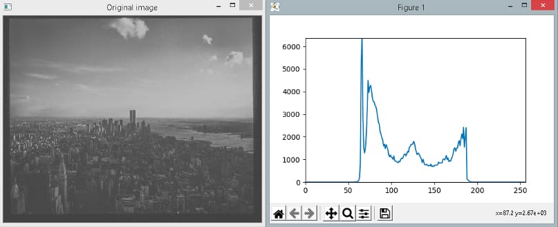
In the above example, we read the img2.jpeg image in the grayscale format. Then, we calculate its histogram using the cv2.calcHist() method. We provide the input image and pass [0] for channels argument as it is a grayscale image. We provide None for the mask argument because we want to plot the histogram of the complete image. Moreover, we pass 256 for the histSize as we want to display the frequency of each pixel separately. After calculating the histogram, we plot it using the method plt.plot() function. Moreover, we use plt.xlim() and plt.ylim() functions to set the limits for the x-axis and the y-axis, respectively. Finally, we use the plt.show() method to display the plot.
If we look at the histogram, we can observe that it is a low contrast image because the pixel values are limited to a specific range only, i.e., the difference between the maximum intensity value and the minimum intensity value is small.
Let’s now plot histograms of the following colored image.

import cv2
import matplotlib.pyplot as plt
img = cv2.imread("img4.jpg")
color = ('b','g','r')
cv2.imshow("Original image", img)
for i,col in enumerate(color):
    hist = cv2.calcHist([img],[i], None, [256], [0, 256])
    plt.plot(hist, color=col)
plt.show()
cv2.waitKey(0)
cv2.destroyAllWindows()
Output
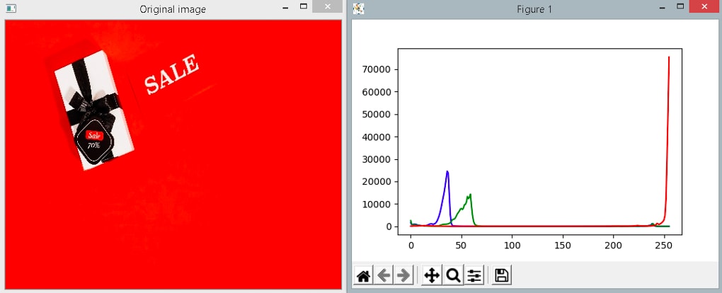
In the above example, the histogram for each channel is shown in the corresponding color. As you can observe, the image mostly contains the red color, which is also evident from the histogram as the frequency of red is a lot.
Let’s consider another colored image.
import cv2
import matplotlib.pyplot as plt
img = cv2.imread("img5.jpg")
color = ('b','g','r')
cv2.imshow("Original image", img)
for i,col in enumerate(color):
    hist = cv2.calcHist([img],[i], None, [256], [0, 256])
    plt.plot(hist, color=col)
plt.show()
cv2.waitKey(0)
cv2.destroyAllWindows()
Output
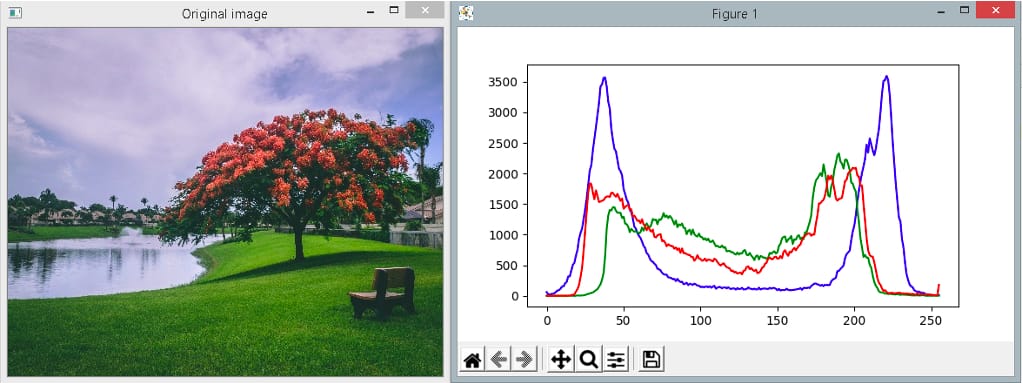
In the above example, the image has both the dark and bright regions. Therefore, histograms for all three channels have higher frequencies on the two ends.
Histogram Equalization
In the first example of the above section, we plotted the histogram of a low contrast image. We observed that the range of the pixel values was limited to a specific region only. Similarly, for dark images, the range of pixel values will be confined to the lower part of the x-axis. Such images have large peaks. A better image, on the other hand, has pixel values distributed across the whole region. Histogram equalization is used to achieve that. It is a technique that improves the contrast and normalizes the brightness of an image by spreading the peaks of the histogram across the whole region.
The cv2.equalizeHist() function equalizes the histogram of a grayscale image. It takes the source image as an input and returns a histogram equalized image.
Let’s apply it to the low contrast image used in the above section.
import cv2
import matplotlib.pyplot as plt
img = cv2.imread("img2.jpeg",0)
equalized_img = cv2.equalizeHist(img)
hist = cv2.calcHist([img],[0], None, [256], [0, 256])
equalized_hist = cv2.calcHist([equalized_img],[0], None, [256], [0, 256])
fig, ax = plt.subplots(2, 2, figsize=(9,7))
ax[0, 0].plot(hist)
ax[0,0].set_title("Histogram of the original image")
ax[0, 1].plot(equalized_hist)
ax[0,1].set_title("Equalized histogram")
ax[1, 0].imshow(img, cmap="gray")
ax[1, 0].set_title("Original image")
ax[1, 1].imshow(equalized_img, cmap="gray")
ax[1,1].set_title("Histogram equalized image")
plt.show()
Output
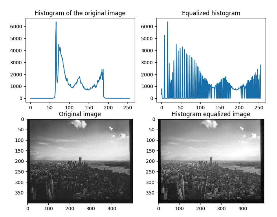
As you can see in the output above, the pixel values are stretched across the whole range when we apply histogram equalization. In the above example, code lines from 7 to 16 plot histograms and images. Here is a separate picture of the histogram equalized image so you can see the difference.
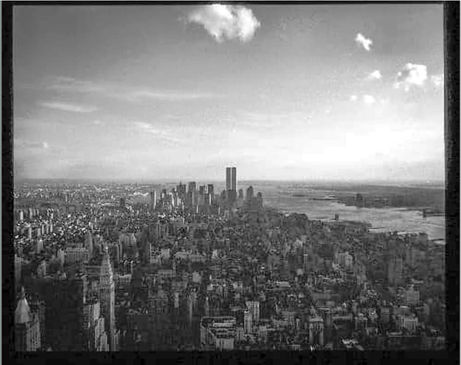
As you can observe, the contrast is increased.
So, how will we apply histogram equalization to a colored picture (RGB or BGR) since cv2.equalizeHist() only takes an image with one channel? One approach might be to equalize each channel separately. However, the results obtained from this can be erroneous. What we can do is convert the image to the HSV format, apply the histogram equalization on the intensity (value) or the saturation channel, and convert it back to the RGB (or the BGR) format.
Let’s apply histogram equalization to the following image.

import cv2
import matplotlib.pyplot as plt
img = cv2.imread("im3.jpeg")

img_hsv = cv2.cvtColor(img, cv2.COLOR_BGR2HSV)
img_hsv_equalized = img_hsv
img_hsv_equalized[:,:,2] = cv2.equalizeHist(img_hsv[:,:,2])
equalized_img = cv2.cvtColor(img_hsv_equalized, cv2.COLOR_HSV2BGR)

cv2.imshow("original image", img)
cv2.imshow("equalized image", equalized_img)

fig, ax = plt.subplots(1, 2, figsize=(11,5))
hist = cv2.calcHist([img],[2], None, [256], [0, 256])
ax[0].plot(hist)
ax[0].set_title("Histogram of the original image, Value Channel")
equalized_hist = cv2.calcHist([img_hsv_equalized], [2], None, [256], [0, 256])
ax[1].plot(equalized_hist)
ax[1].set_title("Equalized histogram, Value Channel")

plt.show()
cv2.waitKey(0)
cv2.destroyAllWindows()
Output
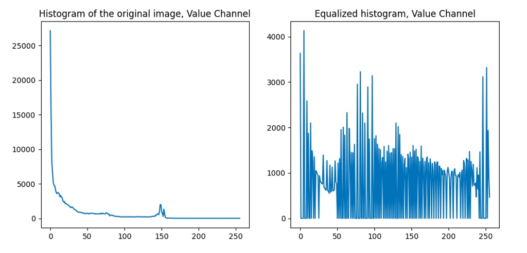
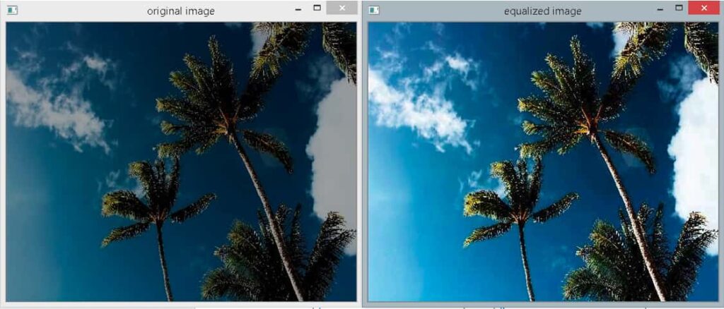
As you can see, the given input image is dark. To resolve this issue, we will have to apply histogram equalization on the value channel. Therefore, first, we convert the image to the HSV format. After that, we equalize the third (value) channel and then convert it back to BGR. The above output shows original and enhanced images and their histograms.
If the image is too bright, then we will have to equalize the saturation channel. Let’s see.

import cv2
import matplotlib.pyplot as plt
img = cv2.imread("im1.jpeg")

img_hsv = cv2.cvtColor(img, cv2.COLOR_BGR2HSV)
img_hsv_equalized = img_hsv
img_hsv_equalized[:,:,1] = cv2.equalizeHist(img_hsv[:,:,1])
equalized_img = cv2.cvtColor(img_hsv_equalized, cv2.COLOR_HSV2BGR)

cv2.imshow("original image", img)
cv2.imshow("equalized image", equalized_img)

fig, ax = plt.subplots(1, 2, figsize=(11,5))
hist = cv2.calcHist([img],[1], None, [256], [0, 256])
ax[0].plot(hist)
ax[0].set_title("Histogram of the original image, Saturation Channel")
equalized_hist = cv2.calcHist([img_hsv_equalized], [1], None, [256], [0, 256])
ax[1].plot(equalized_hist)
ax[1].set_title("Equalized histogram, Saturation Channel")

plt.show()
cv2.waitKey(0)
cv2.destroyAllWindows()
Output
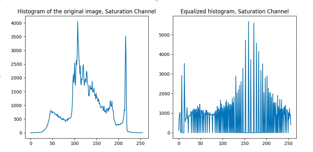

That’s all about Image Histograms in OpenCV Python! 😊


