
Image Thresholding in Python Using OpenCV
in Python, Image Processing on November 19, 2020by coseriesThresholding is another main topic in image processing and computer vision. It is used in image segmentation, i.e., separating the foreground from its background. In this article, we will look at different thresholding techniques and how they are different from one another.
Simple (Global) Thresholding
It is the most basic and straightforward technique. Here, all the pixels having values greater than the threshold value are assigned a single value, for example, 255, and all the other pixels are given some other value, for example, 0.
Simple, right? But how do you find the threshold value? We can approximate it from the histogram of the image or find it through trial and error. A histogram is used to visualize the intensity distribution of an image. It contains pixel value on the x-axis and its frequency on the y-axis. If the foreground and the background of the image are well-separated, then you can approximate the threshold value by choosing a point that separates the two histograms peaks.
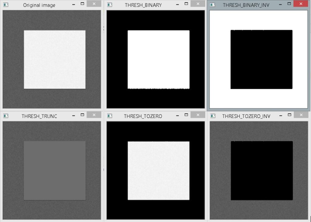
OpenCV provides the cv2.threshold() function for global thresholding. It takes a grayscale image, threshold value, maximum value that can be assigned to a pixel, and a flag for the thresholding type. OpenCV provides several thresholding types, which are given below:
- cv2.THRESH_BINARY: pixel values greater than the threshold value are assigned the maximum value specified in the function. Otherwise, they are assigned 0.
- cv2.THRESH_BINARY_INV: This is the inverse of the cv2.THRESH_BINARY. If the pixel value is greater than the threshold value, it is assigned 0, else the maximum value.
- cv2.THRESH_TRUNC: If the pixel value is greater than the threshold, it is assigned the threshold value. Otherwise, the value remains the same.
- cv2.THRESH_TOZERO: Here, all the pixels having values greater than the threshold value stay the same, and the remaining ones become 0.
- cv2.THRESH_TOZERO_INV: This is the inverse of the cv2.THRESH_TOZERO.
The cv2.threshold() function outputs a retVal and the thresholded image. We will see what is retVal later.
Let’s apply simple thresholding to the following image.

import cv2


img = cv2.imread("dog.jpg", 0)
img = cv2.resize(img, (500, 400))
retVal,dst = cv2.threshold(img,135,255,cv2.THRESH_BINARY)
cv2.imshow("Original image", img)
cv2.imshow("thresholded image Image", dst)
cv2.waitKey(0)
cv2.destroyAllWindows()
Output
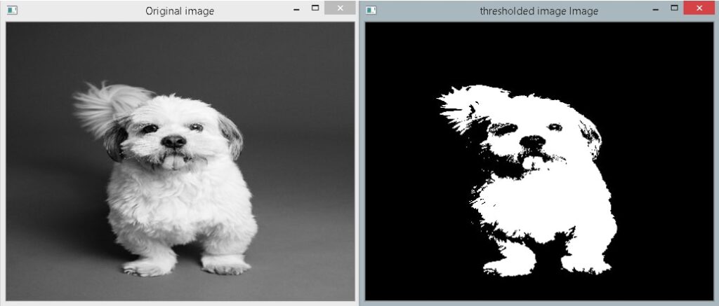
In the above example, first, we load the image in the grayscale format. Then, we resize it to 400×500 dimensions, so it is easier for us to see the image in the window. After that, we apply the cv2.threshold() function. Here the threshold value is 135, which is found by analyzing the histogram and trial and error method. (You will learn about histograms in the later article). Moreover, the thresholding type used is cv2.THRESH_BINARY. Finally, we display the grayscale image and the segmented image.
Let’s now look at the results of other thresholding types.
import cv2

img = cv2.imread("shape_img.jpg", 0)
img = cv2.resize(img, (300, 300))
retVal,thresh_binary = cv2.threshold(img,155,255,cv2.THRESH_BINARY)
retVal,thresh_binary_inv = cv2.threshold(img,120,255,cv2.THRESH_BINARY_INV)
retVal,thresh_trunc = cv2.threshold(img,120,240,cv2.THRESH_TRUNC)
retVal,thresh_tozero = cv2.threshold(img,129,255,cv2.THRESH_TOZERO)
retVal,thresh_tozero_inv= cv2.threshold(img,120,255,cv2.THRESH_TOZERO_INV)
cv2.imshow("Original image", img)
cv2.imshow("THRESH_BINARY", thresh_binary)
cv2.imshow("THRESH_BINARY_INV", thresh_binary_inv)
cv2.imshow("THRESH_TRUNC", thresh_trunc)
cv2.imshow("THRESH_TOZERO", thresh_tozero)
cv2.imshow("THRESH_TOZERO_INV", thresh_tozero_inv)
cv2.waitKey(0)
cv2.destroyAllWindows()
Output
Adaptive Thresholding
In the above thresholding technique, we used one value for the whole image, i.e., a global threshold. The problem with this method is it assumes that the whole image would be uniform. However, often, this is not the case. For example, an image can have different lighting conditions in various regions. In such a scenario, a better approach would be to calculate a threshold value for a specified region instead of the whole image. Thus, we will have multiple threshold values corresponding to various areas of the image. This type of thresholding is known as the adaptive thresholding. The cv2.adaptiveThreshold() function performs the adaptive thresholding. It takes an image, maximum value that can be assigned to a pixel, adaptive thresholding method, thresholding type, neighborhood size, and a constant C. There are two adaptive thresholding methods:
- cv2.ADAPTIVE_THRESH_MEAN_C: The threshold value is calculated as the mean of the given neighborhood minus the constant C.
- cv2.ADAPTIVE_THRESH_GAUSSIAN_C: Here, the threshold value is the Gaussian weighted sum of the given neighborhood minus C.
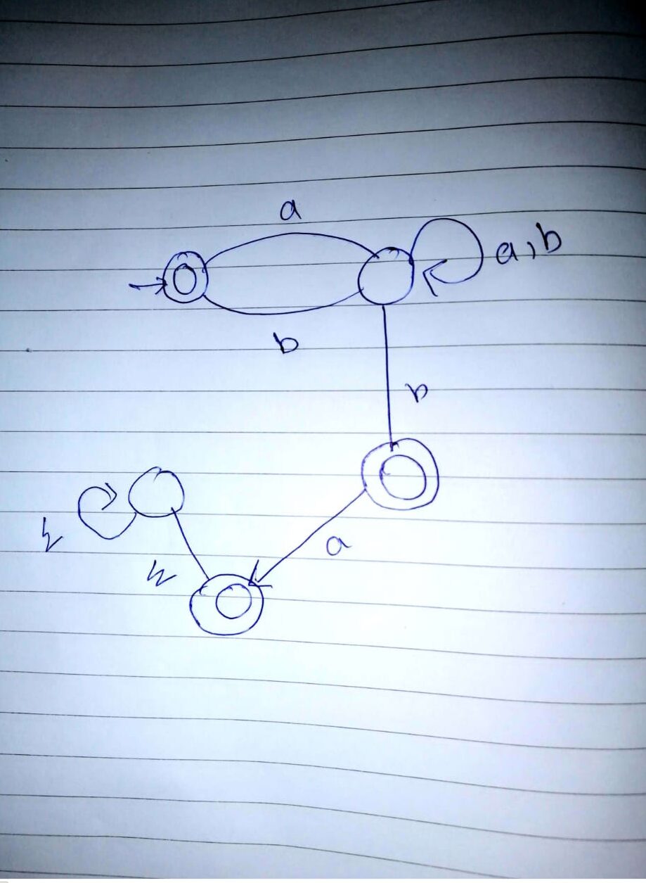
Let’s apply the global and adaptive thresholding on the following image, which has different lighting effects.
import cv2

img = cv2.imread("page3.jpeg", 0)
img = cv2.resize(img, (500, 400))
retVal,simple_thresh = cv2.threshold(img,127,255,cv2.THRESH_BINARY)
adaptive_thesh_mean = cv2.adaptiveThreshold(img, 255, cv2.ADAPTIVE_THRESH_MEAN_C, cv2.THRESH_BINARY, 7, 4)
adaptive_thesh_gaussian = cv2.adaptiveThreshold(img, 255, cv2.ADAPTIVE_THRESH_GAUSSIAN_C, cv2.THRESH_BINARY, 7, 4)

cv2.imshow("Original image", img)
cv2.imshow("Simple Threshold", simple_thresh)
cv2.imshow("Adaptive Threshold Mean", adaptive_thesh_mean)
cv2.imshow("Adaptive Threshold Gaussian", adaptive_thesh_gaussian)

cv2.waitKey(0)
cv2.destroyAllWindows()
Output
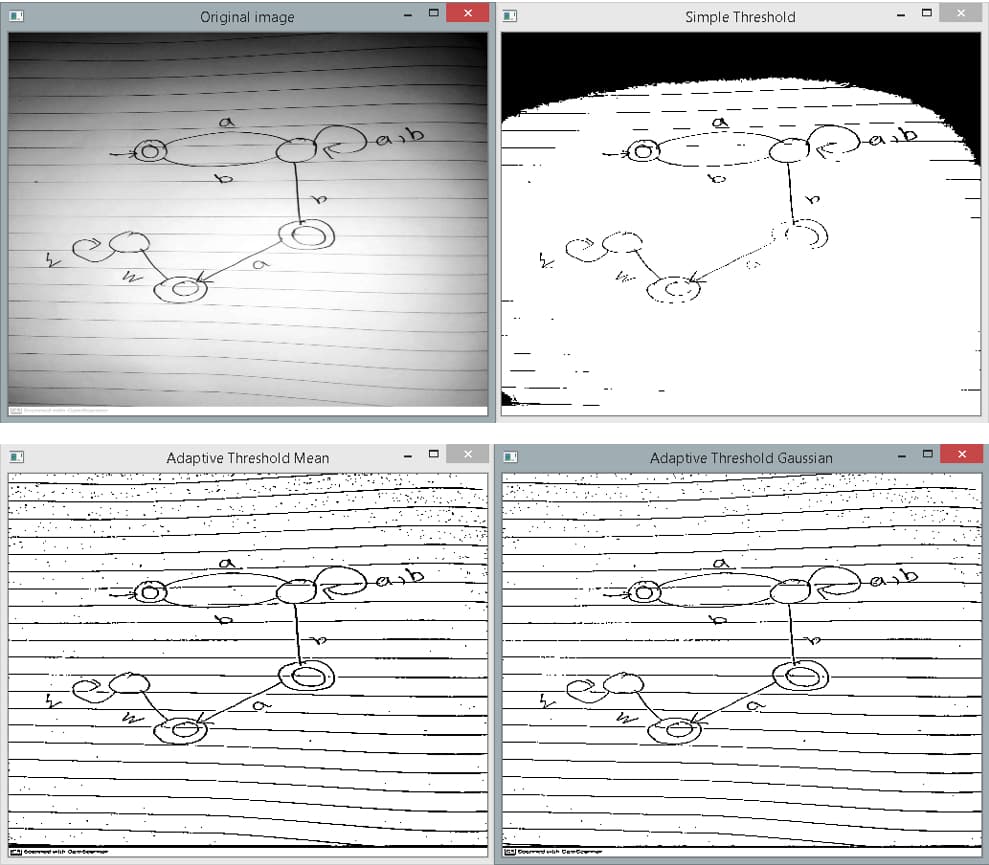
As you can see in the output above, results obtained from the adaptive thresholding are a lot better than the simple thresholding. Moreover, as you can observe, Gaussian thresholding performs better than the mean thresholding.
Otsu’s Binarization
The global thresholding technique has two downsides. First, we have to manually find the threshold value by trial and error method and analyzing the histogram. Second, the value obtained will be approximate and might not be optimal. Otsu’s binarization saves us this trouble and automatically finds an optimal threshold value. However, it works on the assumption that the image is bimodal, i.e., its histogram has two peaks. If it is not, then the threshold value might not be optimal.
To apply Otsu’s thresholding, use the cv2.threshold() function. However, we have to pass an additional flag cv2.THRESH_OTSU. Moreover, pass 0 as the threshold value. Remember, cv2.threshold() outputs retVal and the thresholded image. The retVal contains the threshold value calculated by Otsu’s binarization. If you use the simple thresholding technique, then it will be the same value that you provided as an argument. Consider the example below.
import cv2
img = cv2.imread("sea_img.jpg", 0)
img = cv2.blur(img, (27, 27))
img = cv2.resize(img, (500, 400))
retVal,otsu_thresh = cv2.threshold(img,0,255,cv2.THRESH_BINARY+cv2.THRESH_OTSU)
print(f"Threshold Value: {retVal}")
cv2.imshow("Original image", img)
cv2.imshow("OTSU's Binarization", otsu_thresh)

cv2.waitKey(0)
cv2.destroyAllWindows()
Output
Threshold Value: 151.0
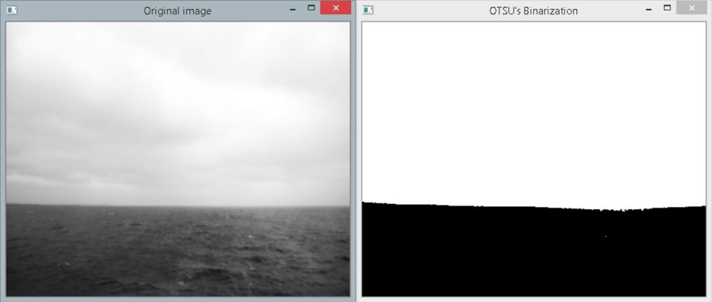
Note that if the image is noisy or not bimodal, Otsu’s binarization might not work well. So, if there is a noise, first, try to remove it using smoothing filters and then apply the thresholding.
import cv2
from matplotlib import pyplot as plt
img = cv2.imread("shape_noise.jpg", 0)
img = cv2.resize(img, (500, 400))
ret2,otsu_thresh = cv2.threshold(img,0,255,cv2.THRESH_BINARY+cv2.THRESH_OTSU)
cv2.imshow("Original image", img)
cv2.imshow("OTSU's Binarization", otsu_thresh)
plt.hist(img.ravel(),256,[0,256])
plt.show()
cv2.waitKey(0)
cv2.destroyAllWindows()
Output

In the above example, we have a noisy image, and Otsu’s binarization does not provide us an effective result, as you can see above. Moreover, code lines 8 and 9 are used to plot the histogram of the shape_noise.jpg image. As you can observe, the intensity distribution is not bimodal.
plt.hist(img.ravel(),256,[0,256])
plt.show()
Let’s reduce the noise using the median filter and apply the Otsu’s method again.
import cv2
from matplotlib import pyplot as plt
img = cv2.imread("shape_noise.jpg", 0)
img = cv2.medianBlur(img, 15)
img = cv2.resize(img, (500, 400))
ret2,otsu_thresh = cv2.threshold(img,0,255,cv2.THRESH_BINARY+cv2.THRESH_OTSU)
cv2.imshow("Smoothened image", img)
cv2.imshow("OTSU's Binarization", otsu_thresh)
plt.hist(img.ravel(),256,[0,256])
plt.show()
cv2.waitKey(0)
cv2.destroyAllWindows()

Here, we apply a median filter of size 15 by 15 to remove the noise, and as you can see, Otsu’s thresholding performs a lot better now.


