Geometric Transformations in Python using OpenCV

In our previous article of this series, we learnt about Arithmetic and Bitwise Operations on Image. In this article we are going to discuss on Geometric Transformations.
Geometric transformations such as scaling, translation, and rotation are quite important and have a lot of applications. For example, you need to resize the image to a specific size according to the need of your application. Rotation is also widely used. A simple example is a rotation feature for your photos on your phones. Moreover, when it comes to training a computer vision model, it requires a lot of image data. Sometimes, that amount of data is not available. So, you apply various kinds of transformations, including geometric transformations, on the available images to increase data. This is known as data augmentation. In this article, we will cover different geometric transformations with examples using OpenCV.

The Transformation Matrix

A transformation can be expressed as:

P’  = A P

where

P’ = [x’, y’, 1] in the homogenous coordinate, or [x’, y’] otherwise. It represents the new position after applying the transformation. It is a column matrix.

P = [x, y, 1] in the homogenous coordinate, or [x, y] otherwise. It is a column matrix, and it represents the original position. A = [[a₁₁, a₁₂, a₁₃], [a₂₁, a₂₂, a₂₃], [0,  0, 1]]. It is a 3×3 matrix in the homogenous coordinate, or 2×3 otherwise. Matrix A is known as the Affine Matrix or the Transformation Matrix. The variables a₁₁, a₁₂, and a₁₃, etc. will have different values according to the transformation applied. So, let’s see each one of them one by one.

Scaling

Scaling is the resizing of the image. We can either scale up (increase the size of an image) or scale down (decrease the size).

Scaling using the cv2.resize() function

To perform scaling, we can use the cv2.resize() function. It takes an image, the tuple containing the new width and the height, i.e., (width, height). Instead of providing the new size, you can provide the scaling factor as well. Since resizing either scales up or scales down an image, OpenCV provides different interpolation methods to fill the gaps. Some important methods are given below:

• cv2.INTER_LINEAR – It is the default interpolation method and preferred for upscaling an image.
• cv2.INTER_CUBIC – It is also preferred for upscaling an image. Since it is computationally complex, so it is slower than cv2.INTER_LINEAR. However, the results are better.
• cv2.INTER_AREA – It is a preferred method for downscaling an image.

Overall, the function becomes cv2.resize(img, (width, height), fx, fy, interpolation).

Let’s resize the following flower image.

import cv2
import numpy as np

img1 = cv2.imread("flower.jpg")
height, width, ch = img1.shape
print(f"Original size: {img1.shape}")
result = cv2.resize(img1, (2*width, 1*height))
print(f"New size: {result.shape}")
cv2.imshow("Result",result)
cv2.imshow("flower", img1)
cv2.waitKey(0)
cv2.destroyAllWindows()

Output

Original size: (500, 400, 3)
 New size: (500, 800, 3)

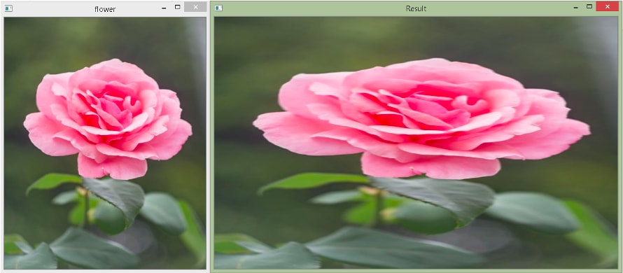
In the example above, first, we read the flower.jpg image. We store its height and width in variables. Then, we use the cv2.resize() method. The newly resized image will have the width two times the original width, and the height will be the same. We use the default interpolation method here.

Consider the following code, where we pass scaling factors instead of the width and the height.

import cv2
import numpy as np

img1 = cv2.imread("flower.jpg")
height, width, ch = img1.shape
print(f"Original size: {img1.shape}")
result = cv2.resize(img1, None, fx = 2, fy = 1)
print(f"New size: {result.shape}")
cv2.imshow("Result",result)
cv2.imshow("flower", img1)
cv2.waitKey(0)
cv2.destroyAllWindows()

Output

Original size: (500, 400, 3)
 New size: (500, 800, 3)

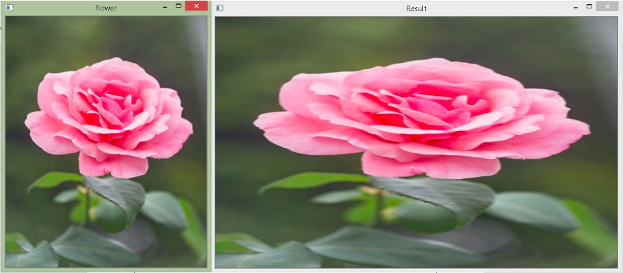
Here, in the cv2.resize() function, we pass None as the second argument because we want to give scaling factors. We pass fx = 2, which means scaling every x-coordinate(column)  by the factor of 2, and we pass fy = 1, which means that we are not changing the y-coordinate(row). The final width will be 800 because the last x is at 400, so 2×400 = 800.

Scaling using the cv2.warpAffine() function

If we talk about the affine matrix for scaling, it is:

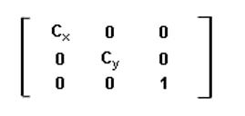
Here, C_x is the scaling factor for the column pixels(width), and C_y is the scaling factor for the row pixels(height).

What it does is multiplies each (x, y) location by C_x and C_y, i.e.,

x’ = C_x × x

y’ = C_Y × y

To perform geometric transformations, we can use OpenCV’s warpAffine() method. It takes three required arguments. The first argument is the image on which we want to apply the transformation. The second argument is a 2×3 transformation matrix, and the third argument is a tuple containing the size in the order (width, height).

Note that warpAffine() takes a 2×3 matrix instead of a 3×3 matrix. Therefore, we need to exclude the last row in the affine matrix given above.

Consider the following example.

import cv2
import numpy as np

img1 = cv2.imread("flower.jpg")
height, width, ch = img1.shape
print(f"Original size: {img1.shape}")
cx = 2;
cy = 1;
affine_matrix = np.float32([[cx,0,0],[0,cy,0]])
result = cv2.warpAffine(img1, affine_matrix, (cx*width, cy*height))
print(f"New size: {result.shape}")
cv2.imshow("Result",result)
cv2.imshow("flower", img1)
cv2.waitKey(0)
cv2.destroyAllWindows()

Output

Original size: (500, 400, 3)
 New size: (500, 800, 3)

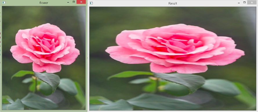
In the above example, we create the transformation matrix using the np.float32() method. The array needs to be of the type float. Here, C_x = 2 and C_y = 1. Then, we call the cv2.warpAffine() method to perform the scaling.

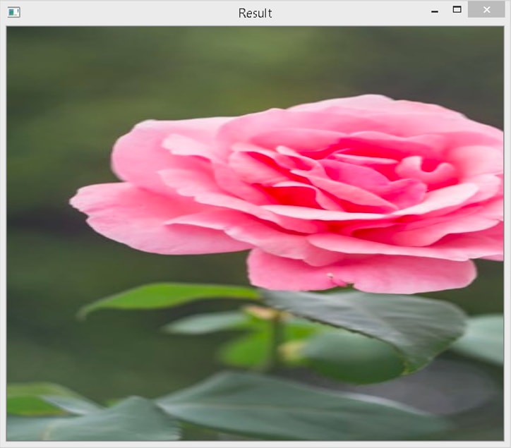
As you can see, this gives the same output as the cv2.resize() function. However, you need to pass the final size explicitly in the warpAffine() method. If you provide a size that is greater than what would be obtained by the transformation matrix, then the remaining portion will be black. If you give a smaller size, then your rescaled image will get cropped. Let’s see.

The rescaled image obtained when you pass 600 for height in the warpAffine() method in the above example. The remaining portion is black.

The rescaled image obtained when you pass 600 for width in the warpAffine() method in the above example. The rescaled image gets cropped.

Translation

The translation is the shifting of an image. In translation, the image size does not change, but the pixels are moved from its original location to another location. The affine matrix for translation is:

Here, t_x and t_y represent the shift along the x (column) direction and the y(row) direction, respectively.

x’ = x + t_x

y’ = y + t_Y

Translation can be done using the cv2.warpAffine() method. Let’s see.

import cv2
import numpy as np

img1 = cv2.imread("flower.jpg")
height, width, ch = img1.shape
tx = 20;
ty = 20;
affine_matrix = np.float32([[1,0,tx],[0,1,ty]])
result = cv2.warpAffine(img1, affine_matrix, (width, height))
cv2.imshow("Result",result)
cv2.imshow("flower", img1)
cv2.waitKey(0)
cv2.destroyAllWindows()

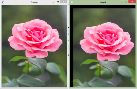
In the above example, we shift each pixel in the image to 20 pixels to the right and 20 pixels to the bottom. We have provided the same width and height as the original image. Therefore, it gets cropped.

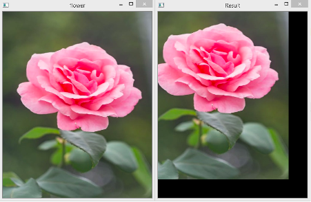
If we assign negative numbers to t_x and t_y, the image will shift in the opposite direction, i.e., to the left and the top. Let’s see.

Rotation

The affine matrix for rotation is:

Where α is the angle of rotation

x’ = xcosα – ysinα

y’ = xsinα + ycosα

Let’s see how we can do it using the cv2.warpAffine() method.

import cv2
import numpy as np
import math
img1 = cv2.imread("flower.jpg")
height, width, ch = img1.shape
alpha = 10;
cos = math.cos(math.radians(alpha))
sin = math.sin(math.radians(alpha))
affine_matrix = np.float32([[cos,-sin,0],[sin,cos,0]])
result = cv2.warpAffine(img1, affine_matrix, (width, height))
cv2.imshow("Result",result)
cv2.imshow("flower", img1)
cv2.waitKey(0)
cv2.destroyAllWindows()

Output

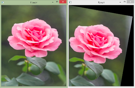
In the above example, we rotate the image by 10^o. We use the math module to calculate sine and cosine values. Moreover, they take angles in radians. Therefore, we use the math.radians() method to convert degrees to radians. The width and height are the same as the original image.

Let’s now rotate it by 90^o.

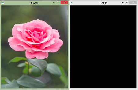
As you can observe, you are not able to see the rotated image because the center of rotation is at (0,0), and thus, the rotated image does not fit.

The cv2.getRotationMatrix2D() function

OpenCV provides a function cv2.getRotationMatrix2D() to get the transformation matrix that will rotate an image with an adjustable center of rotation, and the image can be rescaled as well to fit into the given size. The cv2.getRotationMatrix2D() takes a tuple to specify the center of rotation, angle in degrees, and uniform (isotropic) scaling factor. Moreover, positive angle values represent the counterclockwise direction.

Let’s see.

import cv2

img1 = cv2.imread("flower.jpg")
height, width, ch = img1.shape
alpha = 90
affine_matrix = cv2.getRotationMatrix2D((width/2,height/2),alpha,1)
result = cv2.warpAffine(img1, affine_matrix, (width, height))
cv2.imshow("Result",result)
cv2.imshow("flower", img1)
cv2.waitKey(0)
cv2.destroyAllWindows()

Output

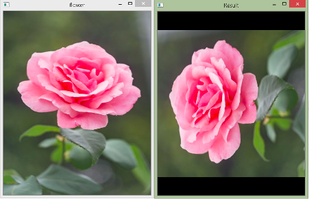
In the above example, we put the center of rotation at the image center. The angle of rotation is 90^o and no scaling factor, i.e., 1. As you see in the output above, it gets rotated nicely.

Consider the same example as above, except the angle is 60^o and the scaling factor is 0.7.

import cv2

img1 = cv2.imread("flower.jpg")
height, width, ch = img1.shape
alpha = 60
affine_matrix = cv2.getRotationMatrix2D((width/2,height/2),alpha,0.6)
result = cv2.warpAffine(img1, affine_matrix, (width, height))
cv2.imshow("Result",result)
cv2.imshow("flower", img1)
cv2.waitKey(0)
cv2.destroyAllWindows()

Output

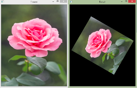
That’s all for this article. Awesome, right? In our next article, we will learn about image smoothing.